<?xml version="1.0" encoding="utf-8"?><feed xmlns="http://www.w3.org/2005/Atom" ><generator uri="https://jekyllrb.com/" version="3.10.0">Jekyll</generator><link href="https://naren219.github.io/feed.xml" rel="self" type="application/atom+xml" /><link href="https://naren219.github.io/" rel="alternate" type="text/html" /><updated>2026-05-13T21:07:21+00:00</updated><id>https://naren219.github.io/feed.xml</id><title type="html">Naren Manikandan</title><subtitle>Personal site</subtitle><entry><title type="html">neural network weight prediction</title><link href="https://naren219.github.io/blog/neural-pred/" rel="alternate" type="text/html" title="neural network weight prediction" /><published>2026-05-11T00:00:00+00:00</published><updated>2026-05-11T00:00:00+00:00</updated><id>https://naren219.github.io/blog/neural-pred</id><content type="html" xml:base="https://naren219.github.io/blog/neural-pred/"><![CDATA[<p><strong>TL;DR</strong>: I tried two related tasks: predicting an MLP’s outputs from its weights (easy — works with concat or residual nets), and the inverse problem of inferring weights from input-output pairs (harder — required moving to a Deep Sets architecture, where the bottleneck shifts from sample count to model capacity).</p>

<hr />

<p>I wanted to build a simple neural network to do a slightly tricky task: can we predict the weights of the model from just the inputs and outputs? Part I walks through a simpler task of confirming that we can simulate a forward pass from a certain architecture, and <a href="#part-ii">Part II</a> will delve into the question above.</p>

<h2 id="part-i">Part I</h2>

<p>We have a well-defined task: given inputs and weights of another, smaller neural net, can we predict its outputs with this network? Since the function defined by the generator net (smaller one) is well-defined and continuous, by <a href="https://en.wikipedia.org/wiki/Universal_approximation_theorem">Universal approximation theorem (UAT)</a>, a sufficiently large ReLU net (nonlinearities are key) can approximate it. The theorem guarantees that this is possible, but provides no details for how to do it. So let’s do it.</p>

<h3 id="architecture">Architecture</h3>

<p>To keep things concise, we’ll define two layers with a ReLU activation for our data generator. We can easily pass in weight tensors and evaluate any input.</p>

<div class="language-py highlighter-rouge"><div class="highlight"><pre class="highlight"><code><span class="k">def</span> <span class="nf">get_mlp_out</span><span class="p">(</span><span class="n">x</span><span class="p">,</span> <span class="n">w1</span><span class="p">,</span> <span class="n">w2</span><span class="p">):</span>
  <span class="n">y1</span> <span class="o">=</span> <span class="n">F</span><span class="p">.</span><span class="n">relu</span><span class="p">(</span><span class="n">x</span> <span class="o">@</span> <span class="n">w1</span><span class="p">)</span>
  <span class="k">return</span> <span class="n">y1</span> <span class="o">@</span> <span class="n">w2</span>
</code></pre></div></div>

<p>
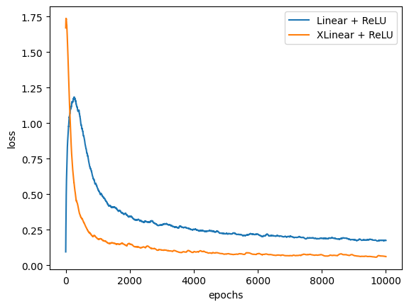
The predictor net has two network variations we’ll compare.</p>

<div class="language-py highlighter-rouge"><div class="highlight"><pre class="highlight"><code><span class="k">class</span> <span class="nc">XLinear</span><span class="p">(</span><span class="n">nn</span><span class="p">.</span><span class="n">Module</span><span class="p">):</span>
  <span class="k">def</span> <span class="nf">forward</span><span class="p">(</span><span class="bp">self</span><span class="p">,</span> <span class="n">x</span><span class="p">):</span>
    <span class="n">h</span> <span class="o">=</span> <span class="n">x</span>

    <span class="k">for</span> <span class="n">layer</span> <span class="ow">in</span> <span class="n">layers</span><span class="p">:</span>
      <span class="n">h</span> <span class="o">=</span> <span class="n">activation</span><span class="p">(</span><span class="n">layer</span><span class="p">(</span><span class="n">h</span><span class="p">))</span>
      <span class="n">h</span> <span class="o">=</span> <span class="n">concat</span><span class="p">(</span><span class="n">h</span><span class="p">,</span> <span class="n">x</span><span class="p">)</span>  <span class="c1"># reattach original input each time
</span>
    <span class="k">return</span> <span class="n">output_layer</span><span class="p">(</span><span class="n">h</span><span class="p">)</span>
</code></pre></div></div>

<p><code class="language-plaintext highlighter-rouge">XLinear</code> has strength over a plain Linear network because the generator input and weights that we concatenate at each layer can skip information bottlenecks from previous hidden layers.</p>

<p>To provide even more scaffolding, we’ll also look at <code class="language-plaintext highlighter-rouge">ResLinear</code> (it doesn’t actually have any conv layers like a typical ResNet, but maybe the skip connections would still help).</p>

<div class="language-py highlighter-rouge"><div class="highlight"><pre class="highlight"><code><span class="k">class</span> <span class="nc">ResBlock</span><span class="p">(</span><span class="n">nn</span><span class="p">.</span><span class="n">Module</span><span class="p">):</span>
  <span class="k">def</span> <span class="nf">forward</span><span class="p">(</span><span class="bp">self</span><span class="p">,</span> <span class="n">x</span><span class="p">):</span>
    <span class="k">return</span> <span class="n">activation</span><span class="p">(</span><span class="n">main_path</span><span class="p">(</span><span class="n">x</span><span class="p">)</span> <span class="o">+</span> <span class="n">skip_path</span><span class="p">(</span><span class="n">x</span><span class="p">))</span>


<span class="k">class</span> <span class="nc">ResLinear</span><span class="p">(</span><span class="n">nn</span><span class="p">.</span><span class="n">Module</span><span class="p">):</span>
  <span class="k">def</span> <span class="nf">forward</span><span class="p">(</span><span class="bp">self</span><span class="p">,</span> <span class="n">x</span><span class="p">):</span>
    <span class="n">x</span> <span class="o">=</span> <span class="n">input_layer</span><span class="p">(</span><span class="n">x</span><span class="p">)</span>
    <span class="n">x</span> <span class="o">=</span> <span class="n">res_block</span><span class="p">(</span><span class="n">x</span><span class="p">)</span>
    <span class="n">x</span> <span class="o">=</span> <span class="n">res_block</span><span class="p">(</span><span class="n">x</span><span class="p">)</span>
    <span class="k">return</span> <span class="n">output_layer</span><span class="p">(</span><span class="n">x</span><span class="p">)</span>
</code></pre></div></div>

<p>The x samples are the concatenation of the generator net’s input and weight tensors and the y samples are the evaluated output (using <code class="language-plaintext highlighter-rouge">get_mlp_out</code>).</p>

<h3 id="results">Results</h3>

<p>After training with a batch size of 1024 and 50000 training steps, we get the following (note: all the loss curves below use exponential moving average to smooth out the noise).</p>

<p><img src="/assets/images/posts/neuralpred/xlin-comp.png" alt="Comparing XLinear to Linear" /></p>

<p>The concatenation technique did work! But <code class="language-plaintext highlighter-rouge">ResLinear</code> did even better.</p>

<p><img src="/assets/images/posts/neuralpred/xvsres.png" alt="Comparing XLinear to ResLinear" /></p>

<p>
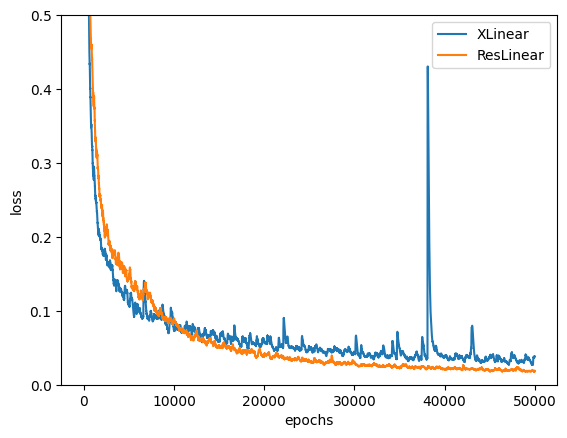
By the end of the training run, we reach a loss of 0.017! This loss can’t be memorization since we sample fresh generator inputs and weights at each batch.</p>

<hr />
<h2 id="part-ii">Part II</h2>

<p>To reiterate: can we build a weight predictor by taking in the inputs and outputs of a generator network?</p>

<p>My first instinct is to try doing the same thing as above and see what results we get. Before that, a few comments – the possible number of weight matrix combinations is massive. how do we incentivize the bigger network to learn the structure of the smaller one. With sufficient I/O samples, would the smaller model’s architecture be the least lossy path?</p>

<p>To begin, let’s first try a much simpler generator net with only one linear layer.</p>

<div class="language-py highlighter-rouge"><div class="highlight"><pre class="highlight"><code><span class="k">def</span> <span class="nf">get_simple_data</span><span class="p">(</span><span class="n">num_unknowns</span><span class="p">,</span> <span class="n">num_pairs</span><span class="p">):</span>
  <span class="c1"># weights are the unknowns
</span>  <span class="n">w</span> <span class="o">=</span> <span class="n">torch</span><span class="p">.</span><span class="n">randn</span><span class="p">(</span><span class="n">batch_size</span><span class="p">,</span> <span class="n">num_unknowns</span><span class="p">,</span> <span class="mi">1</span><span class="p">)</span>
  <span class="n">pairs</span> <span class="o">=</span> <span class="p">[]</span>
  <span class="c1"># we take multiple pairs for each input 
</span>  <span class="c1"># to give more info about the weight layer
</span>  <span class="k">for</span> <span class="n">i</span> <span class="ow">in</span> <span class="nb">range</span><span class="p">(</span><span class="n">num_pairs</span><span class="p">):</span>
    <span class="n">x</span> <span class="o">=</span> <span class="n">torch</span><span class="p">.</span><span class="n">randn</span><span class="p">(</span><span class="n">batch_size</span><span class="p">,</span> <span class="n">num_unknowns</span><span class="p">)</span>
    <span class="n">y</span> <span class="o">=</span> <span class="n">torch</span><span class="p">.</span><span class="n">bmm</span><span class="p">(</span><span class="n">x</span><span class="p">.</span><span class="n">unsqueeze</span><span class="p">(</span><span class="mi">1</span><span class="p">),</span> <span class="n">w</span><span class="p">).</span><span class="n">squeeze</span><span class="p">(</span><span class="mi">1</span><span class="p">)</span>
    <span class="n">pairs</span><span class="p">.</span><span class="n">append</span><span class="p">(</span><span class="n">x</span><span class="p">)</span>
    <span class="n">pairs</span><span class="p">.</span><span class="n">append</span><span class="p">(</span><span class="n">y</span><span class="p">)</span>

  <span class="c1"># ...
</span></code></pre></div></div>

<p>Using this data generator, we should expect that our model (we used <code class="language-plaintext highlighter-rouge">ResLinear</code>) should perform better when given more equations (<code class="language-plaintext highlighter-rouge">num_pairs</code>) than unknowns (<code class="language-plaintext highlighter-rouge">num_unknowns</code>) since the system is overdetermined. So we try this out:</p>

<p><img src="/assets/images/posts/neuralpred/simple-io-pair-comp.png" alt="Comparing three pairs with five pairs with three unknowns (simple generator)" /></p>

<p>
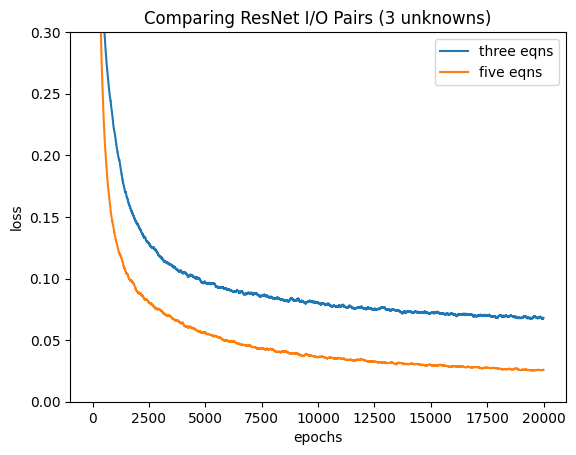
And it worked! The model with five I/O pairs for each weight tensor performed much better. As the network is purely linear, the unknowns can be solved purely by least-squares, so this test is more of a sanity check.</p>

<p>Now, we move onto a more complex generation network that isn’t purely linear.</p>

<div class="language-py highlighter-rouge"><div class="highlight"><pre class="highlight"><code><span class="k">def</span> <span class="nf">get_data_v2</span><span class="p">(</span><span class="n">num_pairs</span><span class="p">):</span>
  <span class="s">"""
  30 pairs for 15 unknowns (2*5+5*1).
  """</span>
  <span class="n">w1</span> <span class="o">=</span> <span class="n">torch</span><span class="p">.</span><span class="n">randn</span><span class="p">(</span><span class="n">batch_size</span><span class="p">,</span> <span class="mi">2</span><span class="p">,</span> <span class="mi">5</span><span class="p">)</span>
  <span class="n">w2</span> <span class="o">=</span> <span class="n">torch</span><span class="p">.</span><span class="n">randn</span><span class="p">(</span><span class="n">batch_size</span><span class="p">,</span> <span class="mi">5</span><span class="p">,</span> <span class="mi">1</span><span class="p">)</span>
  <span class="n">pairs</span> <span class="o">=</span> <span class="p">[]</span>
  <span class="k">for</span> <span class="n">i</span> <span class="ow">in</span> <span class="nb">range</span><span class="p">(</span><span class="n">num_pairs</span><span class="p">):</span>
    <span class="n">x</span> <span class="o">=</span> <span class="n">torch</span><span class="p">.</span><span class="n">randn</span><span class="p">(</span><span class="n">batch_size</span><span class="p">,</span> <span class="mi">2</span><span class="p">)</span>
    <span class="n">y</span> <span class="o">=</span> <span class="n">batch_mlp</span><span class="p">(</span><span class="n">x</span><span class="p">,</span> <span class="n">w1</span><span class="p">,</span> <span class="n">w2</span><span class="p">)</span>  <span class="c1"># MLP generator defined above
</span>    <span class="n">pairs</span><span class="p">.</span><span class="n">append</span><span class="p">(</span><span class="n">x</span><span class="p">)</span>
    <span class="n">pairs</span><span class="p">.</span><span class="n">append</span><span class="p">(</span><span class="n">y</span><span class="p">)</span>

  <span class="n">inp</span> <span class="o">=</span> <span class="n">torch</span><span class="p">.</span><span class="n">cat</span><span class="p">(</span><span class="nb">tuple</span><span class="p">(</span><span class="n">pairs</span><span class="p">),</span> <span class="mi">1</span><span class="p">)</span>
  <span class="c1"># ...
</span></code></pre></div></div>

<p>Training loop:</p>
<div class="language-py highlighter-rouge"><div class="highlight"><pre class="highlight"><code><span class="n">optimizer</span> <span class="o">=</span> <span class="n">torch</span><span class="p">.</span><span class="n">optim</span><span class="p">.</span><span class="n">Adam</span><span class="p">(</span><span class="n">model</span><span class="p">.</span><span class="n">parameters</span><span class="p">(),</span> <span class="n">lr</span><span class="o">=</span><span class="mf">1e-3</span><span class="p">)</span>
<span class="n">loss</span> <span class="o">=</span> <span class="n">nn</span><span class="p">.</span><span class="n">MSELoss</span><span class="p">()</span>

<span class="k">for</span> <span class="n">i</span> <span class="ow">in</span> <span class="n">t</span><span class="p">:</span>
  <span class="n">x</span><span class="p">,</span> <span class="n">weights</span> <span class="o">=</span> <span class="n">get_data_v2</span><span class="p">(</span><span class="n">num_pairs</span><span class="o">=</span><span class="mi">30</span><span class="p">)</span>
  <span class="n">optimizer</span><span class="p">.</span><span class="n">zero_grad</span><span class="p">()</span>

  <span class="n">x_eval</span> <span class="o">=</span> <span class="n">torch</span><span class="p">.</span><span class="n">randn</span><span class="p">(</span><span class="n">batch_size</span><span class="p">,</span> <span class="mi">2</span><span class="p">)</span>

  <span class="c1"># eval true weights on x_eval
</span>  <span class="n">w1</span><span class="p">,</span> <span class="n">w2</span> <span class="o">=</span> <span class="n">weights</span>
  <span class="n">y</span> <span class="o">=</span> <span class="n">batch_mlp</span><span class="p">(</span><span class="n">x_eval</span><span class="p">,</span> <span class="n">w1</span><span class="p">,</span> <span class="n">w2</span><span class="p">)</span>

  <span class="c1"># get weight predictions from test x
</span>  <span class="n">weight_pred</span> <span class="o">=</span> <span class="n">model</span><span class="p">(</span><span class="n">x</span><span class="p">)</span>

  <span class="c1"># eval predicted weights on x_eval
</span>  <span class="n">y_pred</span> <span class="o">=</span> <span class="n">compute_weights</span><span class="p">(</span><span class="n">x_eval</span><span class="p">,</span> <span class="n">weight_pred</span><span class="p">)</span>

  <span class="n">output</span> <span class="o">=</span> <span class="n">loss</span><span class="p">(</span><span class="n">y_pred</span><span class="p">,</span> <span class="n">y</span><span class="p">)</span>
  <span class="n">output</span><span class="p">.</span><span class="n">backward</span><span class="p">()</span>
  <span class="n">optimizer</span><span class="p">.</span><span class="n">step</span><span class="p">()</span>
</code></pre></div></div>
<p>We naively apply the same model to this task. However, there are key modifications to the training procedure:</p>
<ol>
  <li>The loss isn’t computed between the predicted and actual weights. Doing such would make the training incredibly inefficient since there are many valid weight tensors that can implement the same function and we don’t need the exact sequence of them. Essentially, we’re optimizing for <strong>functional equivalence</strong>.</li>
  <li>The loss is computed between the true y – which is outputted from our generator net – and predicted y – which is the result of running a newly-sampled eval x sample through the predicted weights. This is a Monte Carlo estimate of the expected error over the entire input distribution.</li>
</ol>

<p>Turns out, despite having 2x the equations as unknowns, loss doesn’t decrease at all. A few reasons why:</p>
<ol>
  <li>Since we blindly smush the xy pairs into a 1D list in <code class="language-plaintext highlighter-rouge">get_data_v2</code>, we don’t give the model any inductive biases about the groupings of values. This makes learning the I/O mappings an uphill battle.</li>
  <li>The input tensors aren’t permutation invariant, meaning the same layout of pairs in a different arrangement is a new unseen example for the model (which it shouldn’t be).</li>
  <li>With the nonlinearity in the generator net now (ReLU!), it’s a lot harder for another model to learn (especially with issues 1 and 2 included).</li>
</ol>

<p>Let’s try something else: what if we directly embed x and y into some unified vector and have the model predict weights from here?</p>

<h3 id="architecture-1">Architecture</h3>

<div class="language-py highlighter-rouge"><div class="highlight"><pre class="highlight"><code><span class="k">class</span> <span class="nc">PairEncoder</span><span class="p">(</span><span class="n">nn</span><span class="p">.</span><span class="n">Module</span><span class="p">):</span>
  <span class="k">def</span> <span class="nf">__init__</span><span class="p">(</span><span class="bp">self</span><span class="p">,</span> <span class="n">x_dim</span><span class="p">,</span> <span class="n">y_dim</span><span class="p">,</span> <span class="n">embed_dim</span><span class="p">):</span>
    <span class="nb">super</span><span class="p">().</span><span class="n">__init__</span><span class="p">()</span>
    <span class="bp">self</span><span class="p">.</span><span class="n">net</span> <span class="o">=</span> <span class="n">nn</span><span class="p">.</span><span class="n">Sequential</span><span class="p">(</span>
        <span class="n">nn</span><span class="p">.</span><span class="n">Linear</span><span class="p">(</span><span class="n">x_dim</span> <span class="o">+</span> <span class="n">y_dim</span><span class="p">,</span> <span class="mi">128</span><span class="p">),</span>
        <span class="n">nn</span><span class="p">.</span><span class="n">ReLU</span><span class="p">(),</span>
        <span class="n">nn</span><span class="p">.</span><span class="n">Linear</span><span class="p">(</span><span class="mi">128</span><span class="p">,</span> <span class="mi">256</span><span class="p">),</span>
        <span class="n">nn</span><span class="p">.</span><span class="n">ReLU</span><span class="p">(),</span>
        <span class="n">nn</span><span class="p">.</span><span class="n">Linear</span><span class="p">(</span><span class="mi">256</span><span class="p">,</span> <span class="n">embed_dim</span><span class="p">)</span>
    <span class="p">)</span>

  <span class="k">def</span> <span class="nf">forward</span><span class="p">(</span><span class="bp">self</span><span class="p">,</span> <span class="n">x</span><span class="p">,</span> <span class="n">y</span><span class="p">):</span>
    <span class="n">pair</span> <span class="o">=</span> <span class="n">torch</span><span class="p">.</span><span class="n">cat</span><span class="p">([</span><span class="n">x</span><span class="p">,</span> <span class="n">y</span><span class="p">],</span> <span class="n">dim</span><span class="o">=-</span><span class="mi">1</span><span class="p">)</span>
    <span class="k">return</span> <span class="bp">self</span><span class="p">.</span><span class="n">net</span><span class="p">(</span><span class="n">pair</span><span class="p">)</span>
</code></pre></div></div>

<p>Now, we have a pair encoder that transforms a concatenated x and y into an embedding vector.</p>

<div class="language-py highlighter-rouge"><div class="highlight"><pre class="highlight"><code><span class="k">class</span> <span class="nc">WeightPredictor</span><span class="p">(</span><span class="n">nn</span><span class="p">.</span><span class="n">Module</span><span class="p">):</span>
  <span class="k">def</span> <span class="nf">__init__</span><span class="p">(</span><span class="bp">self</span><span class="p">,</span> <span class="n">x_dim</span><span class="p">,</span> <span class="n">y_dim</span><span class="p">,</span> <span class="n">out_dim</span><span class="p">,</span> <span class="n">embed_dim</span><span class="p">):</span>
    <span class="nb">super</span><span class="p">().</span><span class="n">__init__</span><span class="p">()</span>
    <span class="bp">self</span><span class="p">.</span><span class="n">encoder</span> <span class="o">=</span> <span class="n">PairEncoder</span><span class="p">(</span><span class="n">x_dim</span><span class="p">,</span> <span class="n">y_dim</span><span class="p">,</span> <span class="n">embed_dim</span><span class="p">)</span>
    <span class="bp">self</span><span class="p">.</span><span class="n">decoder</span> <span class="o">=</span> <span class="n">nn</span><span class="p">.</span><span class="n">Sequential</span><span class="p">(</span>
        <span class="n">nn</span><span class="p">.</span><span class="n">Linear</span><span class="p">(</span><span class="n">embed_dim</span><span class="p">,</span> <span class="mi">256</span><span class="p">),</span>
        <span class="n">nn</span><span class="p">.</span><span class="n">ReLU</span><span class="p">(),</span>
        <span class="n">nn</span><span class="p">.</span><span class="n">Linear</span><span class="p">(</span><span class="mi">256</span><span class="p">,</span> <span class="mi">128</span><span class="p">),</span>
        <span class="n">nn</span><span class="p">.</span><span class="n">ReLU</span><span class="p">(),</span>
        <span class="n">nn</span><span class="p">.</span><span class="n">Linear</span><span class="p">(</span><span class="mi">128</span><span class="p">,</span> <span class="n">out_dim</span><span class="p">)</span>
    <span class="p">)</span>

  <span class="k">def</span> <span class="nf">forward</span><span class="p">(</span><span class="bp">self</span><span class="p">,</span> <span class="n">x</span><span class="p">,</span> <span class="n">y</span><span class="p">):</span>
    <span class="n">embeddings</span> <span class="o">=</span> <span class="bp">self</span><span class="p">.</span><span class="n">encoder</span><span class="p">(</span><span class="n">x</span><span class="p">,</span> <span class="n">y</span><span class="p">)</span>
    <span class="c1"># avgs across input pairs in each batch. 
</span>    <span class="c1"># key for permutation invariance.
</span>    <span class="n">embed_pooled</span> <span class="o">=</span> <span class="n">embeddings</span><span class="p">.</span><span class="n">mean</span><span class="p">(</span><span class="n">dim</span><span class="o">=</span><span class="mi">1</span><span class="p">)</span>
    <span class="k">return</span> <span class="bp">self</span><span class="p">.</span><span class="n">decoder</span><span class="p">(</span><span class="n">embed_pooled</span><span class="p">)</span>
</code></pre></div></div>

<p>Finally, we decode these embeddings into the weights.</p>

<p>For all the training runs below, we use a learning rate of <code class="language-plaintext highlighter-rouge">1e-3</code> and Lecun weight initialization for the data generator (I didn’t do either in the first iteration and that was a huge mistake). Our embedding dimension has size 128.</p>

<h3 id="results-1">Results</h3>
<p>Following the same paradigm of predicting weights from the train input and using a new eval x to make a y prediction, we get this graph where we try predicting 15 unknowns from the weight layer using 20, 30, and 45 equations.</p>

<p><img src="/assets/images/posts/neuralpred/15-vars-test.png" alt="Predicting 15 unknowns from 20, 30, and 45 eqns" /></p>

<p>
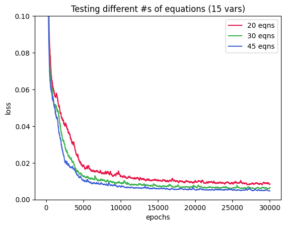
Cool results – our new method works! The loss goes down to 0.005 for the 45 equation curve and only a bit more for the other two plots. Let’s scale up the weights of the generator model and see if we get the same trend.</p>

<p><img src="/assets/images/posts/neuralpred/50-vars-test.png" alt="Predicting 50 unknowns from 67 (🤷‍♂️), 100, and 150 eqns" /></p>

<p>
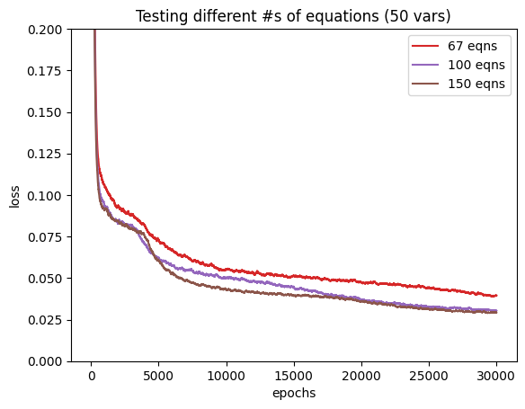
I followed the same scaling factors as before: x1.33, x2, and x3, but with 50 unknowns instead. To compare, let’s use $R^2$, the fraction of variance explained by the model.</p>

$$
\begin{array}{c|cc}
\text{Equations / Unknowns} & \text{15 unknowns} & \text{50 unknowns} \\
\hline
1.33\times & 98.3\% & 91.7\% \\
2\times & 98.6\% & 93.6\% \\
3\times & 99.0\% & 93.8\%
\end{array}
$$

<p>We see that with more unknowns, the problem is genuinely harder per-unit-of-variance, with 5-6% less explained variance at each ratio. Also, there’s saturation from 2x to 3x the equations for the 50 unknowns problem but we still see improvements with the 15 unknowns counterpart. One possible hypothesis for this behavior is the embedding layer bottleneck: the <code class="language-plaintext highlighter-rouge">PairEncoder</code> tries collapsing all pairs into a 128-dim vector. With more unknowns, the same fixed vector needs to hold more information. Furthermore, mean pooling throws away the spread and correlations between pairs which do actually matter – switching to attention pooling could make a huge difference.</p>

<h3 id="discussion">Discussion</h3>

<p>Previously, we raised a question on whether the generator net’s weight layout provides the least-cost option for predicting the right outputs. It’s not clear if the training process results in a weight configuration that falls in the same equivalence class as the true set of weights or the predicted weights happen approximate the function only for this training distribution and not elsewhere. Further tests might include adding more nonlinearities to the generator network or sampling the evaluation x tensors from a different distribution and see if accuracy still holds up.</p>

<p>Turns out, the architecture we used is essentially a <a href="https://arxiv.org/abs/1703.06114">Deep Sets</a> model where we encode the inputs independently, pool across the set, and decode. It’s advantages permutation invariance and the ability to handle input sets of varying sizes. It’s cool that our pretty simple weight prediction challenge independently arrived at the same methods as the paper.</p>

<p>There are many avenues to continue this experiment, from increasing the embedding size to see if it’s the bottleneck to scaling the generator and predictor networks. Checkout the <a href="https://colab.research.google.com/drive/10NUYSQniXh1DWmZ_hkGcCnLoBe_EGyhk?usp=sharing">code</a> and <a href="mailto:nmanikandan219@gmail.com">email me</a> what you think. Thanks!</p>]]></content><author><name></name></author><summary type="html"><![CDATA[TL;DR: I tried two related tasks: predicting an MLP’s outputs from its weights (easy — works with concat or residual nets), and the inverse problem of inferring weights from input-output pairs (harder — required moving to a Deep Sets architecture, where the bottleneck shifts from sample count to model capacity).]]></summary></entry><entry><title type="html">random fun stuff</title><link href="https://naren219.github.io/blog/fun/" rel="alternate" type="text/html" title="random fun stuff" /><published>2026-05-09T00:00:00+00:00</published><updated>2026-05-09T00:00:00+00:00</updated><id>https://naren219.github.io/blog/fun</id><content type="html" xml:base="https://naren219.github.io/blog/fun/"><![CDATA[<p>chillosophy was a club at my high school where we discussed perplexing questions about the world around us. it taught me a lot about the value of conversation and perspective. <a href="https://drive.google.com/drive/folders/11uAVMPeMEsgAtfEWoTdNxrcRLUHVBfvm">here</a> you’ll find all the crazy stuff we talked about.</p>

<p>i wrote my <a href="https://docs.google.com/document/d/1p8M8IcLkv9fGi1V56cmJRlGfHSTW8fANxT8eWPrfaJ8/edit?tab=t.0">personal statement</a> for college about indian astrology. it was quite risky but i tied it into my fascination with the unfathomable and the limits of science.</p>

<p>i love to read. biographies, sci fi, history, philosophy, business: anything i can get my hands on. i have a <a href="https://narenmani.notion.site/1ba8a9a357d2813ea5b9f9b81dc7227e?v=1ba8a9a357d281788add000c530b9586&amp;source=copy_link">notion database</a> tracking the stuff i’ve read and my takeaways from each piece.</p>

<p>things to (maybe) do</p>
<ul>
  <li>understand basic cryptography</li>
  <li>try hacks on raspberry pi</li>
  <li>invest in a crypto currency</li>
  <li>buy an nft (and see how it works)</li>
  <li>try out muzero on some atari game and see how it does</li>
  <li>run alphafold and see how it works</li>
  <li>designing a vision system that can recognize the activity of my parakeets and notify unusual behavior</li>
  <li>try out a ctf</li>
  <li>get a gpu and train a model</li>
  <li>website for dad’s photos</li>
  <li>attend treehacks (and a bunch of hackathons all over the world)</li>
  <li>get into yc (edit: not sure about this)</li>
  <li>go on a sabbatical somewhere remote</li>
  <li>internship at a big tech company (just to see how it looks like to work there)</li>
</ul>]]></content><author><name></name></author><summary type="html"><![CDATA[chillosophy was a club at my high school where we discussed perplexing questions about the world around us. it taught me a lot about the value of conversation and perspective. here you’ll find all the crazy stuff we talked about.]]></summary></entry><entry><title type="html">models of intelligence</title><link href="https://naren219.github.io/blog/intelligence/" rel="alternate" type="text/html" title="models of intelligence" /><published>2026-03-15T00:00:00+00:00</published><updated>2026-03-15T00:00:00+00:00</updated><id>https://naren219.github.io/blog/intelligence</id><content type="html" xml:base="https://naren219.github.io/blog/intelligence/"><![CDATA[<p>i created this article primarily to consolidate my thoughts on how different people have thought of language modeling as a sufficient paradigm for general intelligence.</p>

<p>useful intuitions of language models from <a href="https://www.youtube.com/watch?v=3gb-ZkVRemQ&amp;t=1018s&amp;ab_channel=StanfordOnline">this lecture</a> to preface this piece:</p>

<ul>
  <li>next-token prediction is massively multi-task learning</li>
  <li>scaling compute reliably improves loss</li>
</ul>

<p><strong>in-context learning:</strong> ability for a model to adapt to the user prompt without changing any weights. this leads to zero-shot generalization where the model can answer a novel question in one go based on the patterns and knowledge absorbed during training.</p>

<p>the <strong>residual stream</strong> is an evolving embedding vector that serves as the memory system for the entire model with a deep linear structure (which has many implications in mech interp). attention and feedforward layers can read the embeddings and write to them on every layer, depending on the needs of the model. residual connections preserve past information, serving as a skip connection. this framework shows us that transformers operate on a shared “scratchpad” of embeddings. each layer doesn’t overwrite its predecessor but instead increments the residual stream with whatever new information or feature transformations are needed.</p>

<p>proponents of the “scaling transformers to AGI” paradigm argue that autoregressive predictions of the next token can lead to emergent capabilities when given longer context windows that can represent more complex concepts. models must learn to compress vast amounts of information about the world which correlates with increased generalization.</p>

<p>the pretraining component dismisses most AI scientists from taking this potential path to general intelligence seriously, as the model is ingesting enormous amounts of data and effectively memorizing patterns across the samples. <a href="https://open.substack.com/pub/fchollet/p/how-i-think-about-llm-prompt-engineering">François Chollet states</a> that LLMs store vector programs that map some embedding space to another embedding space, and their reasoning capabilities are only interpolation—bounded by the input data distribution.</p>

<h3 id="chain-of-thought-cot-reasoning">Chain of Thought (CoT) reasoning</h3>

<p>according to this <a href="https://www.interconnects.ai/p/why-reasoning-models-will-generalize">article</a>, compared to direct answer generation where we only rely on a few tokens for processing, we split up the computation between various tokens with CoT prompting. each node gets added to the context window, creating state-space recurrence rather than parameter-space recurrence (the latter exists in a Recurrent Neural Network where this property is built directly into its architecture). recurrence allows the model to adapt to the needs of the prompt and hold a latent representation that it can reuse. likely more links between recurrence and reasoning that i’m missing.</p>

<p>I still feel like the conclusion the author states is lacking explanation (assumption below):</p>

<blockquote>
  <p>chain of thought is a natural fit for language models to “reason” and therefore one should be optimistic about training methods that are designed to enhance it generalizing to many domains.</p>

</blockquote>

<h3 id="reinforcement-learning">reinforcement learning</h3>

<p>it’s pretty amazing what reinforcement learning has allowed us to accomplish. deepseek went from a base V3 model to R1-Zero purely through RL. GRPO was the custom system that rewarded coherence, completeness, and fluency in the model, leading the model to develop the following properties for performance naturally:</p>

<ul>
  <li>reflective behaviors without explicit prompting</li>
  <li>allocate “thinking time” to harder problems and create more CoT traces</li>
  <li>interesting “wait” and “aha” moments that show an understanding of discovery</li>
</ul>

<p>there were still problems with readability and language mixing as Supervised Fine-Tuning was completely excluded. it would be interesting to predict exactly what improvements in the R-zero models would result in domination over the regular R-series. still, this is a massive new frontier as portrayed below.</p>

<blockquote>
  <p>It’s the solving strategies you see this model use in its chain of thought. It’s how it goes back and forth thinking to itself. These thoughts are <em>emergent</em> (!!!) and this is actually seriously incredible, impressive and new (as in publicly available and documented etc.). The model could never learn this with 1 (by imitation), because the cognition of the model and the cognition of the human labeler is different. The human would never know to correctly annotate these kinds of solving strategies and what they should even look like. They have to be discovered during reinforcement learning as empirically and statistically useful towards a final outcome.</p>

  <ul>
    <li>Andrej Karpathy, X</li>
  </ul>
</blockquote>

<p><a href="https://arcprize.org/blog/announcing-arc-agi-2-and-arc-prize-2025">Arc Prize</a> is an amazing effort to continue challenging frontier AI models with a benchmark (Arc-AGI) that’s easy for humans but hard for language models (even reasoning models with the second iteration).</p>]]></content><author><name></name></author><summary type="html"><![CDATA[i created this article primarily to consolidate my thoughts on how different people have thought of language modeling as a sufficient paradigm for general intelligence.]]></summary></entry><entry><title type="html">crypto – notes to self</title><link href="https://naren219.github.io/blog/crypto/" rel="alternate" type="text/html" title="crypto – notes to self" /><published>2026-03-11T00:00:00+00:00</published><updated>2026-03-11T00:00:00+00:00</updated><id>https://naren219.github.io/blog/crypto</id><content type="html" xml:base="https://naren219.github.io/blog/crypto/"><![CDATA[<p><a href="https://bitcoin.org/bitcoin.pdf">bitcoin paper</a></p>

<p>it’s really interesting how bitcoin rethinks our understanding of trust. instead of holding third parties accountable for verifying transactions, bitcoin leverages decentralized consensus to establish a collective truth about the transaction history.</p>

<p>The <strong>Byzantine generals problem</strong> arose from the scenario where a set of generals had to coordinate an attack with the possibilities of message interference and evil generals sabotaging plans. the unsolved issue was that these generals had to be semi-trusted and not completely anonymous for the case of a truly decentralized currency. If there are no “trusted higher-authorities” or notions of identity, how do we prevent single users from using multiple identities and committing harmful actions (aka a Sybil attack)?</p>

<p><strong>proof of work</strong> is the mechanism proposed by Nakamoto by which we can limit identity based on the ability to compute a hard math puzzle, relying on economic and computational costs to make it prohibitively expensive for malicious actors to launch these attacks. this allows bitcoin to fulfill the <a href="https://en.wikipedia.org/wiki/Byzantine_fault"><strong>Byzantine Fault Tolerance</strong></a>, a property in distributed computing of whether independent computers can achieve consensus despite the possibility of malicious nodes that can introduce false information (Nakamoto Consensus).</p>

<p>without a central figure overseeing where blocks are being added, there’s the possibility of double-spending, where users can spend the same tokens more than once. to prevent this, the timestamp server was created where hashes of previous nodes are contained in the current node (hence the name blockchain). modifying any previous block would mean redoing proof-of-work for all the blocks after it, which is very hard to maintain.</p>

<p>two rules to ensure this is feasible:</p>

<ol>
  <li>miners are incentivized to only build blocks on the longest chain (very likely the valid dataset since the computational power is massive).</li>
  <li>transactions are never final on the blockchain as there could be multiple tree branches in which one could be the honest consensus while the others are attackers trying to outcompete the former. yet, it becomes very costly for a malicious chain to outcompete the valid one. it’s shown below how the probability that an attacker catches up drops exponentially, especially when assuming <code class="language-plaintext highlighter-rouge">p &gt; q</code>.</li>
</ol>

<p><img src="/assets/images/posts/crypto/eqn.jpeg" alt="" /></p>

<p>note: if bad actors control more than 50% of the total computational power, they can dominate consensus, allowing them to double-spend, block transactions, and reorganize chains for their advantage (referred to as a “51% attack”).</p>

<p>incentives for miners are the following:</p>

<ol>
  <li>new coins are added into circulation as miners expend their CPU/GPU time and electricity for mining.</li>
  <li>transaction fees are awarded to miners and paid by users for being able to participate in the network. the exact value operates as a market mechanism where users bid for more prioritization by the miners. most currencies will shift to this form of miner incentives as the number of coins in the blockchain is limited.</li>
</ol>

<p>i wanted to point out this beautiful way that this system disincentivizes bad actors.</p>

<blockquote>
  <p>The incentive may help encourage nodes to stay honest. If a greedy attacker is able to assemble more CPU power than all the honest nodes, he would have to choose between using it to defraud people by stealing back his payments, or using it to generate new coins. He ought to find it more profitable to play by the rules, such rules that favour him with more new coins than everyone else combined, than to undermine the system and the validity of his own wealth.</p>
</blockquote>]]></content><author><name></name></author><summary type="html"><![CDATA[bitcoin paper]]></summary></entry></feed>